Section 1 – Overview
This section establishes a new form of graphical probabilistic representation called an Experiment Graphical Model (EGM).
An EGM is similar to a Probabilistic Graphical Model (PGM). They differ in that the nodes in an EGM are Experiment Results, where in a PGM the nodes are Random Variables. An Experiment Result has all the information of a Random Variable, but adds one more piece of information – the number of samples. This additional information has significant implications:
- experiments with a common sample space and procedure can be combined
- the number of trials in the experiment can be used as an indicator of the significance of an experiment
The Motivation
It is frequently the case where we have results from experiments taken from a same sample space using the same technique but which have different number of trials. We want to combine the results of these experiments while respecting the relative significance represented in the trial counts. Bayes Theorem gives the ability to encode relationships between Random Variables and is commonly used to achieve such an expression. But Bayes Theorem is derived from probabilities, and probabilities do not include the sample count. So Bayes does not have access to sample count, and cannot consider relative significance of the respective sample counts. This limitation of Bayes places an unnecessary handicap in applications where Bayes is applied.
- Given the definition of probability p(A=a1) = nA1 / n (Kolmogorov 1933 set-theoretic definition)
- Bayes chooses to use probability p(A=a1) instead of the more expressive [nA1, n] in its definition.
- where Bayes is p(A=a1|B=b1) = p(B=b1|A=a1) * p(A=a1) / p(B=b1)
In summary: Bayes uses Probability instead of the more expressive [nA1… nAn]. Bayes does not have visibility into the number of events – the “n”. It has thrown away the cardinality of the experiment (the number of trials).
Example 1:
I move from Boston to Irvine. After a month I have experienced 2 earthquakes. One morning I am awoken by a loud noise and shaking. I am extremely confident it is an earthquake. Dr Daphne Koller also lives in that same building and experiences the same loud noise and shaking. She has experienced many earthquakes and is quite confident it is something else.
Given traditional probabilistic representation those evaluations might be Chris: p(quake) = 0.8 Dr Koller: p(quake) = 0.2. But Dr Koller has been living in the area much longer and has more experience detecting earthquakes. She has experienced (say) 934 earthquakes where I have experienced 2. How do we ‘weigh’ degree of experience in combining these? Typically a Bayes network would have random variable nodes “Chris” and “Dr Koller,” and a child node with weights (conditional probabilities) to combine them. The problem is- the degree of confidence that was already part of the original experiments (“2” and “934”) were thrown away in computing the probability. In other words – first we discard “n” after computing p(quake), then we have to create something to replace it – the weight in the child node. It would be preferable to preserve the “n”, and use that in weighing the the relative significance in the child node.
Example 2:
An aeronautic airspeed sensor is a component of an airplane control system that has several such sensors. The sensor expresses its readings in a probabilistic manner P(S=sn) where sn is speed in knots S <is a set containing> (20, 50, 100, 200, 500). Internally, the sensor has access to the temperature and humidity at the sensing point. It may have a heating element and could detect the state of this element. An inherent design element (aperture size) affects its performance. A model, internal to the sensor, factors these parameters in determining the most likely airspeed. The output of the sensor are the five values P(S=sn).
The problem here is the sensor can only express a prediction of airspeed. It cannot express its confidence in that prediction. So, if one sensor is subject to freezing under low temperature/high humidity conditions, it cannot express its low confidence when it detects those conditions. A second sensor optimized for low temperature/high humidity conditions would want to express its strong confidence under those conditions.
We desire a means for the sensor to express not just its airspeed prediction, but also its confidence in that prediction. To do this – we have the sensor express its output as an Experimental Result N(S=sn) where N(S=sn) (is the number of occurrences of that event in an experiment that is equivalent to its current state. That experiment would have the same Procedure, Sample Set, etc ?)
Note the probability P(S=sn) can be earily arrived at as N(S=sn) / card(N) where card(N) = sum_over_n(P(S=sn)
(In the context of the System Controller where we have multiple sensors – if we assume the experiments from those sensors are performed under the same conditions, using the same Procedure, then they can be combined. The output from various sensors can be combined (is the number of occurrences of that event in an experiment that is equivalent to its current state. That experiment would have the same Procedure, Sample Set, etc ?)
In this manner – details of the sensor model are encapsulated within the sensor and not exposed to the system. The sensor is given a means to express its level of confidence to the system. A common and consistent means allows the system to combine results from different sensors.
The Plan
- Define an Experiment Result as triple: Sample Space, Procedure and Collection of Trials.
- We note that Experimental Results establishes a Probability Function, where P(A=a1) = N(A=a1) / N(Sample Space)
- Note that Experiment Results can be combined if they share Sample Space and Procedure. Each Experimental Results can (will) have its own Collection of Trials.
- Express Bayes Theorem using the set-theoretic notation specifically identifying Sample Space and Procedure, but with different Number of Trials.
- Establish Experiment Graphical Model (EGM) – It is the equivalent of a Probabilistic Graphical Model except that it adds a new “Node” – an “Addition” node – where the prerequisite for such node they share Sample Space and Procedure.
- Demonstrate (prove) that any Neural Network can be rewritten as (is) a EGM.
abc
def
Section 2 – Agent and World
Here we introduce the concept (similar to re-enforcement learning) that there is an Agent that interacts with the world.
The parts are:
- Agent – this is our “robot”.
- World – this is the outside world. We assume the external world is causal – that is – there is stimulus and response. We show the cause-effect relationship as downward-flowing (cause is above effect). Stimulus comes from the Agent and is the “cause” and the Response is the “effect”
- Sensors – a sensor interfaces from the World to the Agent and transfers data from the World to the Agent. It is important to note that Sensor is the ultimate “effect” – there are no further downstream effects in the world as a result of a sensor. For example – a sensor may be a CCD array, and the data captured by that array is after all other cause/effects of occlusion, position, shadowning, reflections, illumination, etc etc.
- Actuators – an actuator takes output from the Agent and imparts it to the World. It should be noted that in the World the Actuator is the ultimate Cause, and while there may be other Causes in the World there is nothing upstream of a Cause from an Actuator.
- The PGM or EGM – internal to the Agent – the PGM or EGM is a directed a-cyclic graph (DAG). The nodes of the graph are random variables. At the bottom of the DAG are the a-priori random variables of the PGM which we refer to as “evidence” nodes. The model receives “evidence” from Sensors which are the “effects” observed from the world. The upwards-directed vertices of the graph indicate the dependency relationship of the data – we are given “evidence” from the external world and our graph intends to probabilistically infer the cause from which that effect resulted. It is noted the graph is “upside-down” compared to traditional PGMs – this is done to allow a side-by-side alignment of nodes in the Agent PGM to cause/effect steps in the World.
The diagram below shows an Agent, World, PGM, Sensor and Actuator.
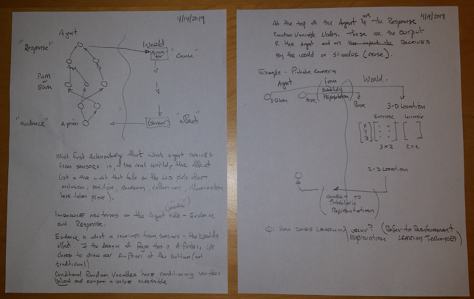
An example is shown above – the pinhole camera. The pinhole camera is a physical entity whereby a point in 3-dimensional space is illuminated, light from that point passes through an infinitely small hole, and the resulting light is projected onto a 2-dimensional surface. The mathematical equation for the transform is <shown in the diagram, but could use LaTex here…>
In this case the World “effect” is the 2-dimensional image. The World “cause” is the 3-dimensional position in space. The camera model has two transforms. The first is the “extrinsic” (a 3-d to 3-d transform) representing the a transform between coordinate spaces – 3-d positions “point space” to 3-d “hole space”. The second transform is the “intrinsic” transform. This is 3-d to 2-d and is the transform from “hole space” to 2-d “image space”.
The Sensor detects the 2-d image and converts to a probabilistic representation <detail here>. The probabilities are given to the Agent and are the values of the bottom-most a-priori nodes in the PGM.
At the “top” of the PGM are the “Response” nodes. Values of these nodes are given to the Actuator block which converts the probabilistic values into absolute positions which are the World “cause”.
Section 3 – Functions, Stochastic Functions, Random Functions, Relations
Recall that a function is a map from a source set to a target set. The source set is the “domain” and the target is the “range” or “co-domain”. The co-domain contains exactly those elements resulting from the function operated on the domain (and no more). A range is a superset of the co-domain (it includes additional elements). Note that the number of elements in a co-domain (it’s cardinality) is less than or equal to that of the domain.
It is important to distinguish between types of functions, because later we will stress our knowledge when we investigate “relations”.
A “traditional function” is deterministic – it consistently maps each element in the domain to exactly one element in the co-domain. A “stochastic function” maps an element in the domain to a specific set of elements in the co-domain according to some probabilistic ratio. A “random function” maps an element in the domain to any element in the co-domain, according to some probabilistic ratio. Note that stochastic function and random function are closely related – the latter is a specific case of the former.
<pictures here would help>
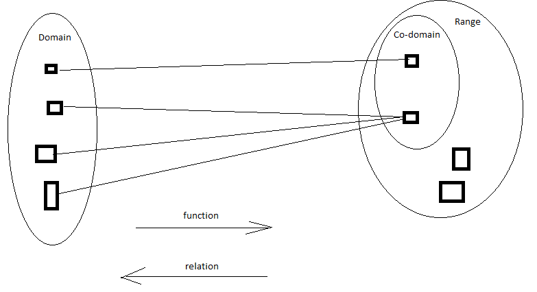
A “relation” is essentially the inverse of a function. In a relation the co-domain is the source, and the relation maps from co-domain to range. Note that a single element in the co-domain may relate to multiple elements in the domain. So for example – the relation corresponding to a “traditional function” is actually a “stochastic function”. I.e. – the relation will map an element in the co-domain to a specific set of elements in the domain. Note also the probability associated with the range mapping is flat – the probability of each specific set of elements is equal (independent of the frequency that the domain element gets chosen).
So – if we are given a ‘traditional function’ this can be modeled using traditional techniques (numeric values). However if we are given a stochastic function, a random function, or a relation – then we need a probabilistic model.